USGS Maps

From: http://biology.usgs.gov/s+t/noframe/image-maps.htm

Home


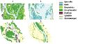
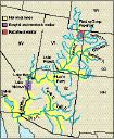
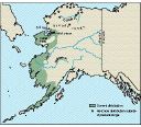
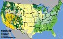
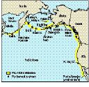
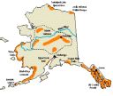
View image

Go to the article

Fig. 3. Alaskan habitats of special importance to geese.

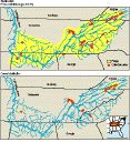
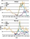
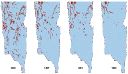
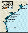
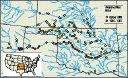
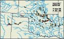
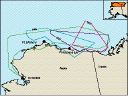
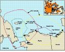
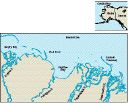
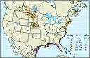
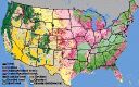
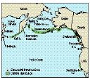
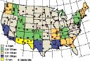
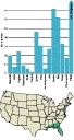
View image

Go to the article

Fig. 2. Location of important staging areas in western North America used by shorebirds during spring and fall migration. Size of dot indicates the estimated peak number of shorebirds at each site.

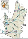
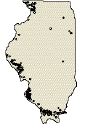
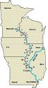
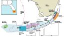
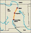
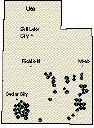
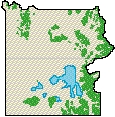
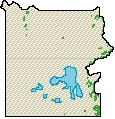
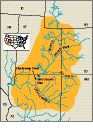
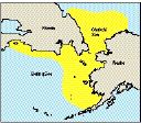
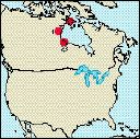
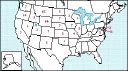
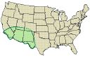
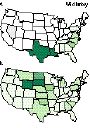
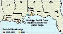
View image

Go to the article

Figure. Range of Mississippi sandhill cranes.

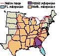
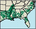
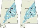
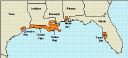
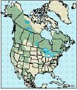
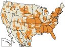
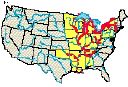
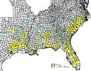
View image

Go to the article

Figure. Distribution of red-cockaded woodpeckers by county and state. Most historical RCW records are cited from Jackson 1971 and Hooper et al. 1980. For information on references, contact R. Costa.

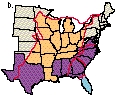
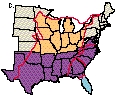
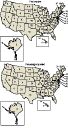
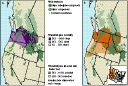
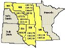
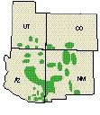
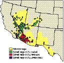
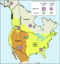
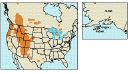
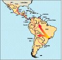
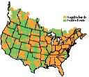
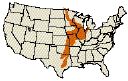
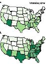
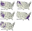
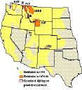
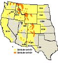
View image

Go to the article

Fig. 1. Approximate distribution of grizzly bears in 1850 compared to 1920 (a; Merriam 1922) and 1970-90 (b). Local extinction dates, by state, appear in (a). Populations identified in (b) are NCE -- North Cascades ecosystem, SE -- Selkirk ecosystem, CYE -- Cabinet-Yaak ecosystem, BE -- Bitterroot ecosystem, NCDE -- Northern Continental Divide ecosystem, GYE -- Greater Yellowstone ecosystem. As indicated in (b), a grizzly was killed in the San Juan Mountains of southern Colorado in 1979.

View image

Go to the article


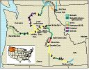
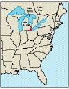
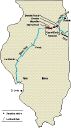
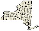
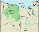
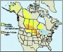
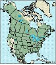
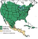
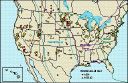
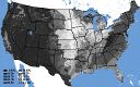
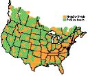
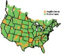
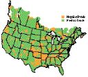
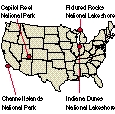
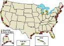
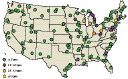
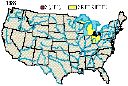
View image

Go to the article

Fig. 1. Range of the Indiana bat and locations of Priority 1 hibernacula (see text for definitions).

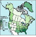
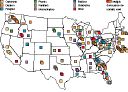
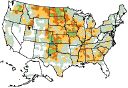
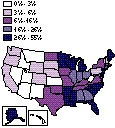
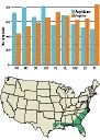
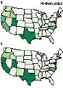
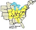
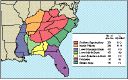
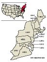
View image

Go to the article

Fig. 2. The harvest of antlered white-tailed deer (number per square mi or 259 ha of deer range) in 13 northeastern states in 1983 (first value) and in 1992 (second value); estimates for Virginia and West Virginia include young-of-the-year males (button bucks).

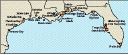
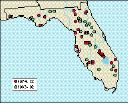
View image

Go to the article

Fig. 1. Locations of survey areas for night-light counts of alligators in Florida, 1974-92.

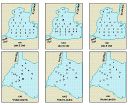
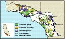
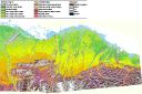
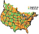
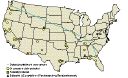
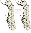
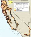
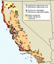
View image

Go to the article

Fig. 1. Historical and current distribution of the northern red-legged frog, California red-legged frog, and Cascades frog in California based on 2,068 museum records and 302 records from other sources. Dots indicate locality records based on verified museum specimens. Squares indicate locality records based on verified sightings (e.g., field notes, photographs, published papers). Red dots and green squares denote localities where native frogs are extant. Gold dots and blue squares indicate where native frogs are presumed extinct. Figure modified from Jennings and Hayes (1993).

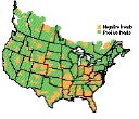
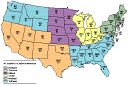
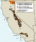
View image

Go to the article

Fig. 2. Historical and current distribution of the foothill yellow-legged frog, spotted frog, and Yavapai leopard frog in California based on 3,316 museum records and 171 records from other sources. Dots indicate locality records based on verified museum specimens. Squares indicate locality records based on verified sightings (e.g., field notes, photographs, published papers). Red dots and green squares denote localities where native frogs are extant. Gold dots and blue squares indicate where native frogs are presumed extinct. Figure modified from Jennings and Hayes (1993).

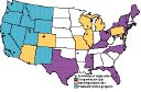
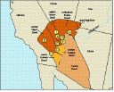
View image

Go to the article

Fig. 3. Historical and current distribution of the mountain yellow-legged frog, and presumed native populations of the northern leopard frog in California based on 2,565 museum records and 673 records from other sources. Dots indicate locality records based on verified museum specimens. Squares indicate locality records based on verified sightings (e.g., field notes, photographs, published papers). Red dots and green squares denote localities where native frogs are extant. Gold dots and blue squares indicate where native frogs are presumed extinct. Figure modified from Jennings and Hayes (1993).

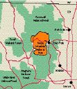
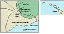
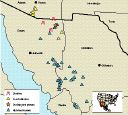
View image

Go to the article

Fig. 1. Range of the Tarahumara frog, Rana tarahumarae. Copper smelters are at Douglas, AZ (now closed), and Cananea and Nacozari, Sonora. Historical locations include both surveyed populations that appeared stable, and unvisited historical localities (Campbell 1931; Little 1940; Williams 1960; Hale et al. 1977; Hale and May 1983; Hale and Jarchow 1988).

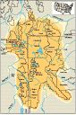
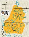
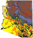
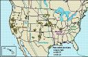
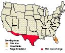
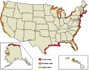
View image

Go to the article

Fig. 1. U.S. range of the desert tortoise (Gopherus agassizii). The six population segments for desert tortoises federally listed as threatened occur in parts of the Mojave and Colorado deserts that lie north and west of the Colorado River.

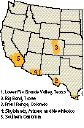
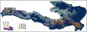
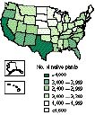
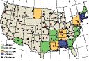
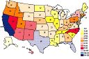
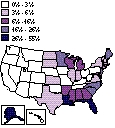
View image

Go to the article

Fig. 1. Total numbers of freshwater fishes and percentage imperiled by hydrographic region of the southeastern United States.

View image

Go to the article

Fig. 3. An example of habitat fragmentation, decline, and isolation of populations of a southeastern freshwater fish, the endangered spotfin chub (Cyprinella monacha). Former (pre-1930's) and present range in yellow.

View image

Go to the article

Figure. Colorado River Basin.

View image

Go to the article

Figure. Distribution and status of white sturgeon in the U.S. portion of the Columbia River Basin.

View image

Go to the article


View image

Go to the article


View image

Go to the article

Figure. Loss of genetic variation among largemouth bass populations. a. The native range of the largemouth bass (Micropterus salmoides) is delineated by the red lines (MacCrimmon and Robbins 1975). As first described by Bailey and Hubbs (1949), the Florida subspecies, M.s. floridanus, was restricted to peninsular Florida (blue); the northern subspecies, M.s. salmoides, covered most of the rest of the range of the species; and there was a relatively small intergrade zone between the two resulting from some indeterminable combination of natural hybridization and human-caused mixing of stocks. b. The expansion of the intergrade by 1980 was described by Philipp et al. (1983). Because detailed ranges were not explored in all states, and because this intergrade zone expansion was likely caused by state stocking programs, entire states are classified according to whether the intergrade zone was expanded. c. The current intergrade zone is now even larger because of the addition of more states in which largemouth bass containing at least some M.s. floridanus genes are being introduced either by the state fish and game agencies themselves or by private groups. Notice that the entire southern and eastern portion of the original range of the northern subspecies, M.s. salmoides, is at risk of being inundated with M.s. floridanus genes.

View image

Go to the article

Fig. 1. Western United States showing five subregions of high species richness.

View image

Go to the article

Figure. Twenty-five major river drainages in Illinois.

View image

Go to the article

Fig. 1. Number of species and subspecies of freshwater mussels historically known to occur within each state and the percentage now classified as imperiled.

View image

Go to the article

Fig. 1. The Lake Huron-Lake Erie corridor, including Lake St. Clair and western Lake Erie (in red).

View image

Go to the article

Fig. 2. Average (mean) densities (number/m2) of native mussels in Lake St. Clair and western Lake Erie of the Lake Huron-Lake Erie corridor of the Great Lakes, 1961-92.

View image

Go to the article

Figure. Distribution of springs and caves in Illinois.

View image

Go to the article

Fig. 1. (a) Natural distribution of whitebark pine (Arno and Hoff 1989; Olgilvie 1990) with mortality zones. Mortality level is the proportion of trees dead from all causes since presettlement. (b) White pine blister rust infection rates in whitebark pine. Blister rust is present but infection rates are unknown in Canada and the southern United States.

View image

Go to the article

Fig. 1. Approximate distribution of forested wetlands along rivers and streams in the southeastern United States prior to European colonization (Putnam et al. 1960).

View image

Go to the article

Fig. 2. Distribution of forested wetlands along the Lower Mississippi River: (a) Precolonial extent based on Putnam et al. (1960); (b) recent extent based on 1982 data (data source: U.S. Fish and Wildlife Service, Vicksburg, Mississippi).

View image

Go to the article

Figure. Abundance of stocked and wild lake trout (Salvelinus namaycush) in Michigan and Wisconsin waters of Lake Superior in 1929-93, expressed as a percentage of the 1929-43 mean (from Hansen et al. 1995).

View image

Go to the article

Fig. 1. Sampling sites for the NBS/USEPA Fish Contaminant Monitoring Program and "hot spots" of sediment contamination where tumors and other deformities have been detected in fish.

View image

Go to the article

Fig. 1. The Upper Mississippi River. Numbers indicate reservoirs formed by navigation dams and known locally as pools.

View image

Go to the article

Fig. 2. Land-cover/land-use comparisons for a portion of Pool 8 in (a) 1891 and (b) 1989, and the open river near Cape Girardeau, Missouri, in (c) 1891 and (d) 1989.

View image

Go to the article

Fig. 3. Island loss that has occurred in Pool 8, in the area just upriver of the dam, since construction of the lock and dam system.

View image

Go to the article

Fig. 1. The Illinois River with locations of navigation locks and dams. Locations of the Illinois Natural History Survey's upper Illinois Waterway electrofishing stations are also shown.

View image

Go to the article

Fig. 2. Historical and current distribution of Tulotoma magnifica. Filled circles represent a single or two closely located collection sites (after Hershler et al. 1990). Map modified from the U.S. Geological Survey 1:500,000 scale--State of Alabama sheet (1970 ed.).

View image

Go to the article

Fig. 1. Landsat Thematic Mapper image of Philadelphia and New York City, taken May 20, 1991.

View image

Go to the article

Figure. Gap analysis of coastal sage scrub in the southwestern region of California. Highlighted are landscapes where coastal sage scrub is the primary and secondary upland vegetation type.

View image

Go to the article


View image

Go to the article

Fig. 1. The 1974 and 1989 Landsat MSS images of Dallas-Fort Worth, Texas. Expanded urban areas are clearly identifiable in the 1989 image and are particularly evident around Dallas-Fort Worth International Airport in the center of the image.

View image

Go to the article

Fig. 2. Landsat MSS images of the Mount Saint Helens area in southern Washington in 1973, 1983, and 1988. The 1973 image shows the area before eruption. The area north of the crater in the image with the bluish color was most devastated by the 1980 eruption. In the 1988 image the light pink color in the blow-out area shows vegetation regrowth.

View image

Go to the article


View image

Go to the article


View image

Go to the article

Fig. 1. The tidal portion of the Hudson River, New York, showing areas where some fish collections have been made over the last six decades.

View image

Go to the article

Fig. 1. The upper, middle, and lower Florida Keys. National marine sanctuaries, national parks, national wildlife refuges, and aquatic preserves are also shown (modified from maps provided by James A. Reed II, Florida Marine Research Institute). Various colors used simply to delineate designated areas.

View image

Go to the article

Fig. 1. Locations of wetland loss study sites along the Gulf of Mexico region.

View image

Go to the article

Fig. 2. Coastal Louisiana basins as defined in the Coastal Wetlands Planning, Protection, and Restoration Act Plan.

View image

Go to the article

Fig. 3. Coastal landloss in Louisiana and elsewhere is analyzed by using computerized geographic information systems that produce graphics such as this map.

View image

Go to the article

Figure. Study sites along the Gulf of Mexico region.

View image

Go to the article

Fig. 1. Major bay systems along the Texas coast.

View image

Go to the article

Fig. 2. Dominant cover types in the continuously submerged portions of upper (a) and lower (b) Laguna Madre.

View image

Go to the article

Figure. The Rio Grande study area.

View image

Go to the article

Fig. 1. New York locations from which phenological data were obtained. 1­Allegheny Plateau (birds); 2­Cayuga Lake basin, Ithaca (birds); and 3­Hudson Highlands (flowering plants and birds).

View image

Go to the article

Figure. Distribution of the original 130 quarter-sections in North Dakota.

View image

Go to the article

Fig. 1. Areas of the Prairie Pothole region and time periods for which estimates of duck nest success were made. See Fig. 2 for abbreviations.

View image

Go to the article

Fig. 1. Historical occurrences of the Arkansas River shiner from collections before 1989 and current occurrences from 1989 to 1991.

View image

Go to the article

Fig. 2. Historical occurrences of the Arkansas River speckled chub from collections before 1992 and current occurrences from 1992 to 1993.

View image

Go to the article

Fig. 1. Distribution of Mexican spotted owls in the southwestern United States.

View image

Go to the article

Fig. 2. Distribution of Mexican spotted owls in canyonlands of southern Utah, representing the northwest portion of the Colorado Plateau Physiographic Province.

View image

Go to the article

Figure. Historical range and current distribution of the three subspecies of desert bighorn in the United States (redrawn from Trefethen 1975 and Weaver 1985).

View image

Go to the article

Fig. 2. Trends in Rocky Mountain National Park visitors, agricultural impacts, moose invasion, elk population, forest recovery, air pollution, Estes Park population, and global change in carbon dioxide.

View image

Go to the article

Fig. 1. Progressively lighter shading is used around the edges of a recent map of the Greater Yellowstone Ecosystem to illustrate the uncertainty that still plagues definitions of the ecosystem. Courtesy Desktop Assistance and Greater Yellowstone Coalition.

View image

Go to the article


View image

Go to the article

Fig. 2. Top: Current distribution of whitebark pine portrayed by a computerized geographic information system (GIS). Bottom: Distribution of whitebark pine projected by GIS analysis under a modest increase in warmth and dryness, showing a decrease of approximately 90%. (Derived from Romme and Turner [1991] by the Yellowstone GIS Laboratory, Yellowstone National Park.)

View image

Go to the article

Fig. 1. Sky island mountain ranges of Arizona, New Mexico, and adjacent Sonora and Chihuahua (Marshall 1957). All of the labeled mountain ranges have pine-oak woodland.

View image

Go to the article

Fig. 1. The Colorado Plateau.

View image

Go to the article

Fig. 3. Historical range and current concentrations of bonytail and razorback sucker (Minckley and Deacon 1991).

View image

Go to the article

Figure. The Colorado Plateau region is cut by dramatic canyons of the Colorado River system.

View image

Go to the article

Fig. 1. Outlines of the annual activity areas for one radio-collared polar bear (Ursus maritimus) monitored during 4 consecutive years. The boundaries of the multiyear activity area enclosed 517,000 km2 (about 200,000 mi2).

View image

Go to the article

Fig. 2. Approximate bounds of the Beaufort Sea and Chukchi Sea polar bear populations. The contours for each population surround 95% and 50% of the radio relocations that were nearest the harmonic mean center of the distribution of relocations.

View image

Go to the article

Figure. Distribution of the tundra hare, with historical records of occurrence outside of its present distribution.

View image

Go to the article

Figure. Distribution of Pacific walruses in the Bering and Chukchi seas of Alaska and Russia (Fay 1982).

View image

Go to the article

Fig. 1. Prudhoe Bay study area showing West Dock and the Endicott Causeway, Alaska.

View image

Go to the article

Fig. 1. Arctic National Wildlife Refuge in northeastern Alaska.

View image

Go to the article

Fig. 2. Land-cover classes on the Arctic National Wildlife Refuge in northeastern Alaska.

View image

Go to the article

Fig. 1. Hawaii Volcanoes National Park, including the Olaa Forest, where population surveys of picture-wing Drosophila have been carried out.

View image

Go to the article

Fig. 3. Known honeybee locations in Arizona displayed with vegetation classes; derived from Brown et al. (1979).

View image

Go to the article

Fig. 1. The Prairie Pothole region and areas sampled in the Breeding Population and Habitat Survey.

View image

Go to the article

Fig. 1. Number of shorebird species regularly breeding and wintering within three broad ecological domains of North America west and east of the Continental Divide (dashed line).

View image

Go to the article

Fig. 1. Historical distribution of the American black bear (modified from Hall 1981).

View image

Go to the article

Fig. 2. Present distribution of the American black bear, based on survey responses from provinces and states (Pelton 1994) and research projects in Mexico (D. Doan, Texas A & I University, personal communication).

View image

Go to the article

Fig. 1. Location of four monitoring sites. Sites chosen represent localities with information for 5 or more years. Site 1­McConnell River (60š 50'N, 94š 25'W; snow goose [Chen caerulescens] and small Canada goose [Branta canadensis]); 2­ La Pérouse Bay (58š 24'N, 94š 24'W; snow goose); 3­Cape Churchill (58š 25'N, 93šW; medium Canada goose); and 4­South-hampton Island (63š 60'N, 86šW; snow goose).

View image

Go to the article

Fig. 2. The proportion of species that would be out of their climate envelope in each state or province with a +3°C (+5.4°F) temperature change.

View image

Go to the article

Fig. 2. Nationwide distribution of lead-poisoned eagles.

View image

Go to the article

Fig. 1. Distribution of the wild turkey in the United States and Mexico in 1989 (Stangel et al. 1992).

View image

Go to the article

Fig. 1. Breeding and wintering ranges of mourning doves and mourning dove management units in the United States.

View image

Go to the article

Figure. Distribution of piping plovers throughout the annual cycle in 1991.

View image

Go to the article

Figure. Distribution of elk in North America as of 1978, based on information provided by provincial and state wildlife agencies (modified from Thomas and Toweill 1982, used with permission, Wildlife Management Institute).

View image

Go to the article

Fig. 2. Known distribution of "western duck sickness" (avian botulism) in North America, 1934 (Kalmback and Gunderson 1934), and from 1975 to 1993.

View image

Go to the article

Fig. 3. Geographic distribution of avian cholera in wild waterfowl within the United States, before 1960 (first outbreak in 1944), during the 1960's, and after 1970, when disease spread (National Wildlife Health Center files).

View image

Go to the article

Fig. 1. Grouped categories of potential natural vegetation aggregated from Küchler (1964).

View image

Go to the article

Fig. 2. Grouped categories of 1990 land cover depicting 1990 conterminous U.S. land cover that was developed from 1990 AVHRR imagery

View image

Go to the article

Fig. 3. Percentage of Küchler's potential natural vegetation types (Küchler 1964) that have been converted to agricultural and urban land cover. The lighter tones represent the higher levels of human modification. Percentages of modification are displayed as deca-percentiles.

View image

Go to the article

Fig. 3. Nationwide distribution of eagle poisonings caused by organophosphorus and carbamate pesticides.

View image

Go to the article

Fig. 1. Origins of the 54 alien species established in Hawaii.

View image

Go to the article

Fig. 2. Dispersal of the 13 breeding visitor species when not breeding.

View image

Go to the article

Fig. 3. Origins of the 155 visitor species that do not breed in Hawaii.

View image

Go to the article

Fig. 2. Coral reef ecosystems under U.S. jurisdiction in the Pacific Ocean. Coral reef ecosystems are found around the northwest and main Hawaiian Islands, Wake Island, Johnston Atoll, Northern Mariana, Guam, Palmyra Island and Kingman Reef, Howland Island, Baker Island, Jarvis Island, and American Samoa. Coral reef ecosystems at risk are indicated by a red asterisk.

View image

Go to the article

Fig. 1a. Distribution of sea otters before fur harvest began in 1741 and populations that survived the harvest, providing the nucleus for recovery of the species. Width of shaded area is not relative to sea otter habitat.

View image

Go to the article

Fig. 1b. Current distribution of sea otters including locations of successful translocations.

View image

Go to the article

Fig. 1. Coral reef ecosystems under U.S. jurisdiction in the western Atlantic Ocean, Gulf of Mexico, and Caribbean Sea. Coral reef ecosystems are found on or around the Florida Reef tract, Flower Garden Banks, Puerto Rico, and U.S. Virgin Islands. Coral reef ecosystems at risk are indicated by an asterisk.

View image

Go to the article

Fig. 1. Migration of Africanized honeybees.

View image

Go to the article

Fig. 1. Geographic patterns in the mean trends for grassland bird species during 1966-92.

View image

Go to the article

Fig. 2. Geographic patterns in the mean trends for shrubland and old-field bird species during 1966-92.

View image

Go to the article

Fig. 3. Geographic patterns in the mean trends for woodland bird species during 1966-92.

View image

Go to the article

Fig. 4. Geographic patterns in the mean trends for Neotropical migrant bird species during 1966-92.

View image

Go to the article

Fig. 5. Geographic patterns in the mean trends for short-distance migrant bird species during 1966-92.

View image

Go to the article

Fig. 6. Geographic patterns in the mean trends for permanent resident bird species during 1966-92.

View image

Go to the article

Fig. 1. Breeding range of Audubon's crested caracara in Florida based on records from 1987 to 1991; range boundaries shown by Howell (1932), and main species' range in western United States.

View image

Go to the article

Fig. 1. Breeding distribution of the southwestern willow flycatcher. Dotted line represents areas where distribution is uncertain.

View image

Go to the article

Figure. Distribution of U.S. endemic amphibian species; those west of the 100th meridian tend to be more broadly dispersed.

View image

Go to the article

Figure. Number of fishes considered imperiled and number of native freshwater fishes of the contiguous United States by state (redrawn from Warren and Burr 1994).

View image

Go to the article

Fig. 1. Distribution of state and local inventories of Lepidoptera in the contiguous 48 United States. States having comprehensive lists (all families) published or in progress, those with macrolepidoptera lists, and those with preliminary lists in progress are indicated. Dots indicate locations of 35 local inventories of single sites, reserves, and islands, either published or in progress.

View image

Go to the article

Fig. 1. Original boundaries of the tall-grass prairie biome in the United States (Risser et al. 1981) and locations of study sites (A.B. Swengel, unpublished data).

View image

Go to the article

Fig. 2. Documented lichen deserts in the United States and Canada. Strong anecdotal evidence exists that lichen deserts also occur in most major cities.

View image

Go to the article

Fig. 1. The number of native vascular plant species in each state.

View image

Go to the article

Fig. 3. The proportion of globally rare vascular plant species (ranked G1, rarest, to G3, more common) in the native flora of each U.S. state.

View image

Go to the article

Fig. 4. The proportion of species reported potentially extirpated from the native flora of each U.S. state.

View image

Go to the article

Fig. 1. Four national park units studied.

View image

Go to the article

Figure. Gross range of presettlement oak savanna in central North America (adapted from Nuzzo 1986 and Smeins and Diamond 1986). The shaded area represents the general region in which oak savannas occurred, although this region was not uniformly savanna. Significant blocks of nonsavanna vegetation, such as prairie or forest, were also present within it. Nor was oak savanna totally restricted to this region. Small, disjunct outliers existed as far east as Ohio and as far west as the Dakotas.

View image

Go to the article

Figure. Classification of annual shoreline change around the United States (modified from U.S. Geological Survey. 1985).

View image

Go to the article

Fig. 1. The National Oceanic and Atmospheric Administration's National Status and Trends Program monitors more than 350 sites nationwide for chemical con-taminants in fish livers, bivalve molluscan tissues, and associated sediments. Yellow symbols depict Mussel Watch Project (molluscan and sediment monitoring) and red symbols depict National Benthic Surveillance Project (fish and sediment monitoring) sites.

View image

Go to the article

Fig. 3. Geographic distribution of DDE residues in starlings collected in 1985. Also shown are boundaries of the 5-degree (latitude and longitude) sampling blocks and collection sites.

View image

Go to the article


View image

Go to the article

Fig. 4. Geographic distribution of PCB residues in U.S. Fish and Wildlife Service monitoring networks: (a) PCB concentrations in fish collected in 1986 from the indicated sites. Not shown are stations in Alaska and Hawaii, at which PCB concentrations were < 1.5 parts per million (ppm) at all sites; (b) PCBs in starlings collected in 1985. Also shown are boundaries of the 5-degree (latitude and longitude) sampling blocks and collection sites.

View image

Go to the article

Fig. 2. Location by state of organophosphorus and carbamate compounds in pesticide-related wildlife mortality incidents, 1980-93.

View image

Go to the article


View image

Go to the article

Fig 1. The number of nonindigenous fish species reported by state, 1800-1994. Some species may not be established or have been eradicated.

View image

Go to the article

Fig. 1. States with zebra mussel sightings in inland or adjacent waters, 1988. In 1989, they spread to Lake Superior, Lake Michigan, and Lake Ontario (National Biological Service, unpublished data).

View image

Go to the article

Fig. 3. States with zebra mussel sightings in inland or adjacent waters in 1993. The range has extended west of the Mississippi River into Oklahoma by way of the Arkansas River (National Biological Service, unpublished data).

View image

Go to the article

Fig. 2. Confirmed presence of Africanized honeybees in (colored) counties of Arizona, New Mexico, and Texas, January 15, 1994.

View image

Go to the article

Fig. 1. Surface-area percentage of wetlands in each state: 1780's (Dahl 1990).

View image

Go to the article

Fig. 2. Surface-area percentage of wetlands in each state: 1980's (Dahl 1990).

View image

Go to the article

Fig. 3. Wetland acreage loss by state (Dahl 1990).

View image

Go to the article

Fig. 4. Surface-area percentage of wetland base loss by state (Dahl 1990).

View image

Go to the article

Fig. 2. Historical distribution of the longleaf pine ecosystem in the southeastern Coastal Plain. Chart shows the present total number of species of amphibians and reptiles in various southeastern states.

View image

Go to the article

Fig. 4. The distribution of the gopher tortoise (Gopherus polyphemus) in the southeastern United States. The chart shows the number of species of various taxa known to use its burrow and the number of plant taxa described from the longleaf pine-wiregrass ecosystem.

View image

Go to the article

Fig. 3. Percentage of 27 birds showing positive and negative trends.

View image

Go to the article

Fig. 1. Range and abundance patterns of the mute swan. (a) Data from 1901 to 1940, (b) Data from 1960 to 1989 (except 1969).

View image

Go to the article

Fig. 2. Range and abundance patterns of the wild turkey. (a) Data from 1901 to 1940, (b) Data from 1960 to 1989 (except 1969).

View image

Go to the article

Fig. 3. Range and abundance patterns of the mourning dove. (a) Data from 1901 to 1940, (b) Data from 1960 to 1989 (except 1969).

View image

Go to the article

Fig. 4. Range and abundance patterns of the barred owl. (a) Data from 1901 to 1940. (b) Data from 1960 to 1989 (except 1969).

View image

Go to the article

Fig. 5. Range and abundance patterns of the bald eagle. (a) Data from 1901 to 1940. (b) Data from 1960 to 1989 (except 1969).

View image

Go to the article

Fig. 6. Maps showing range and abundance patterns of the northern pintail. (a) Data from 1901 to 1940. (b) Data from 1960 to 1989 (except 1969).

View image

Go to the article

Fig. 1. Range of: a --sagebrush steppe; b -- juniper woodlands; c -- ponderosa pine; d -- lodgepole pine; and e -- southern pineland communities in the United States.

View image

Go to the article

Figure. Distribution of purple loosestrife, Asian clam, zebra mussel, and carp in the United States (shading indicates species presence).
*U.S. Congress 1993.
**U.S. Department of the Interior, National Biological Service 1994. Non-native aquatic species data base.

View image

Go to the article

Figure. Distribution of several non-native animal species on public lands as reported by land managers responding to mail surveys: feral cat, wild pig, feral dog, non-native trout, carp, and wild horse.